
#-3 | Guinness Pro12 15/16: A hierarchial model
Recently I read this blog post which looks at applying a hierarchical Bayesian model to understand the uncertainty of the attacking and defensive strengths of different teams in the Six Nations. It is a replication of another blog post which applies the model to data from the English Premier League. The models used by both blogs are based on a paper outlining two such models and applying them to Serie A, the premier division of Italian football.
The league portion of the 15/16 Guinness Pro 12 is now finished. I thought it might be fun to apply the same technique to this data, especially since there are playoffs at the end of the competition consisting of two semi-finals and a final which could be interesting to simulate. Unfortunately I didn’t get this post up before the semi-finals last weekend, but better late than never! Unlike the blog posts above which use python I have done everything in R using JAGS to perform Markov Chain Monte Carlo.
Getting the Data
I expected a good bit of wrangling to get the data I needed but it turned out to be pretty straight forward. On the Pro 12 website I went to the Fixtures and Results section. All the data I needed was there but I haven’t scraped much data from the web in my time. I took a punt and googled something like R html table and found the readHTMLTable function which is a part of the XML package. So I pointed this at the Pro 12 URL in my browser and hoped for the best!
It seemed to return a list containing a NULL object and two dataframes. The dataframes were both quite similar but I just picked one and then went about tidying it up. It’s all shown below.
# If we already have a copy of the tables from the pro12 website don't bother getting them again
# This is here as i'll be regenerating an rmarkdown script a lot while writing this.
table.file <- '~/pro12_readHTMLTable.rds'
if (!file.exists(table.file)) {
  theurl <- "http://www.pro12rugby.com/matchcentre/fixtures_list.php?includeref=10808&season=2015-2016#z8HvpmemZhdCZzOK.97"
  dt.pro12.results <- readHTMLTable(theurl, stringsAsFactors=FALSE)
  saveRDS(dt.pro12.results, table.file)
} else {
  dt.pro12.results <- readRDS(table.file)
}

# Use element 3 of the list, remove NA rows as it's clear that any row with NAs
# is the header from a particular round. Convert to a data.table.
dt.pro12.results <- as.data.table(na.omit(dt.pro12.results[[3]]))
# The column names we want are stuck in the first row so drop it after getting the names.
pro12.col.names <- as.character(unlist(dt.pro12.results[1]))
dt.pro12.results <- dt.pro12.results[-1,]
# If the column name is blank we'll be dropping this column
pro12.col.names[pro12.col.names==''] <- 'drop'
colnames(dt.pro12.results) <- pro12.col.names
dt.pro12.results[,drop := NULL]
dt.pro12.results[,drop := NULL]
# colnames to lower case
setnames(dt.pro12.results,tolower(colnames(dt.pro12.results)))
# having a / in a colname is annoying
setnames(dt.pro12.results,'tv/att','attendence')
# Any row with a v in the score column is a game that hasn't been played yet.
# When the final is over there will be none of these, and the last three games
# will need to be dropped to replicate this analysis.
dt.pro12.results <- dt.pro12.results[score!='v',]
# add home and away score columns. tstrsplit is very handy here.
dt.pro12.results[, c("h", "a") := tstrsplit(score, " - ", type.convert=TRUE)]
dt.pro12.results[,score := NULL]
# Add a game id. Seems wrong not to.
dt.pro12.results[,game.id:=.I]
# Only use the league stages
dt.pro12.results <- dt.pro12.results[1:(12*11)]
# We don't need these details
dt.pro12.results[,date := NULL]
dt.pro12.results[,time := NULL]
dt.pro12.results[,venue := NULL]
dt.pro12.results[,attendence := NULL]
After this we have the following data set consisting of the home and away team names and the score.
##                  home                  away  h  a game.id
##   1:   Connacht Rugby Newport Gwent Dragons 29 23       1
##   2:  Edinburgh Rugby        Leinster Rugby 16  9       2
##   3:     Ulster Rugby               Ospreys 28  6       3
##   4: Glasgow Warriors              Scarlets 10 16       4
##   5:    Munster Rugby      Benetton Treviso 18 13       5
##  ---
## 128:  Edinburgh Rugby         Cardiff Blues 17 21     128
## 129:   Leinster Rugby      Benetton Treviso 50 19     129
## 130:    Munster Rugby              Scarlets 31 15     130
## 131:          Ospreys          Ulster Rugby 26 46     131
## 132:      Zebre Rugby Newport Gwent Dragons 47 22     132
Next I associated a team id with each team and calculate the total points they scored and conceded in the season.
# Come up with team ids
teams <- data.table(team=unique(dt.pro12.results$home))
teams[,team.id:=.I]
# join the team ids to the results table.
setkey(teams,'team')
dt.pro12.results[,home.team.id:=teams[home,team.id]]
dt.pro12.results[,away.team.id:=teams[away,team.id]]
# We don't need the team names anymore
dt.pro12.results[,home := NULL]
dt.pro12.results[,away := NULL]
# add points for and against. This is tricky since each teams points can be in
# the home or away column. There must be a better way to do this!
setkey(dt.pro12.results, home.team.id)
teams[,home.for := dt.pro12.results[,sum(h),by=home.team.id][team.id,V1]]
teams[,home.against := dt.pro12.results[,sum(a),by=home.team.id][team.id,V1]]
setkey(dt.pro12.results, away.team.id)
teams[,away.for := dt.pro12.results[,sum(a),by=away.team.id][team.id,V1]]
teams[,away.against := dt.pro12.results[,sum(h),by=away.team.id][team.id,V1]]
teams[,pts.for := home.for+away.for]
teams[,pts.against := home.against+away.against]
teams[,home.for := NULL]
teams[,home.against := NULL]
teams[,away.for := NULL]
teams[,away.against := NULL]
setkey(teams, team.id)
Now the results table and the teams table look like this
##       h  a game.id home.team.id away.team.id
##   1: 23 28      95            2            1
##   2: 18 10     110            3            1
##   3: 33 32       8            4            1
##   4: 12 18      47            5            1
##   5: 20 16      49            6            1
##  ---
## 128: 13  0       7            7           12
## 129: 20 12      48            8           12
## 130:  8 18      65            9           12
## 131: 52  0      77           10           12
## 132: 36  3      39           11           12
## team team.id pts.for pts.against
## 1: Connacht Rugby 1 507 406
## 2: Edinburgh Rugby 2 405 366
## 3: Ulster Rugby 3 488 307
## 4: Glasgow Warriors 4 557 380
## 5: Munster Rugby 5 459 417
## 6: Cardiff Blues 6 542 461
## 7: Newport Gwent Dragons 7 353 492
## 8: Scarlets 8 477 458
## 9: Benetton Treviso 9 320 614
## 10: Leinster Rugby 10 458 290
## 11: Ospreys 11 490 455
## 12: Zebre Rugby 12 308 718A few spot checks of the pts.for and pts.against columns against the final league table on the Pro12 site confirms all is well. Also the total of each should be equal.
teams[,list(for.total=sum(pts.for), against.total=sum(pts.against))]## for.total against.total
## 1: 5364 5364A scatter plot gives a simple overview of each teams attacking and defensive strength.
ggplot(teams, aes(x=pts.against, y=pts.for)) +
  geom_label(aes(label=team, x=pts.against, y=pts.for),size=4) +
  geom_point(color='blue', alpha=0.5) +
  xlim(c(200, 800)) +
  ylim(c(200, 600)) +
  ggtitle('Pro 12 15/16 points for and against')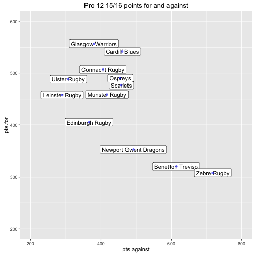
The goal of the remaining analysis is to use the individual game data to understand the uncertainty of these attributes.
Modelling
The model is well described in the links above but I will describe it here as well for completeness. The idea is that each team \(i\) has an underlying attack and defense parameter - \(att_i\) and \(def_i\).
It is assumed that the number of points a team will score in a game is a random variable following a Poisson distribution and its rate parameter is derived from the attacking and defensive strengths of both teams. Let \(p^h_{ij}\) be the number of points scored by the home team in a match between teams \(i\) and \(j\) and let \(p^a_{ij}\) be the number of points scored by the away team. Then
\[p^h_{ij} \sim Poisson(\theta^h_{ij})\] \[p^a_{ij} \sim Poisson(\theta^a_{ij})\]and
\[log(\theta^h_{ij}) = intercept + home\_adv + att_i + def_j\] \[log(\theta^a_{ij}) = intercept + att_j + def_i\]Here \(intercept\) accounts for the number of points you would expect teams to score in a game on average, while \(home\_adv\) accounts for the extra points you might expect the home team to score. Note that the intercept term isn’t included in the paper looking at Serie A.
So when teams \(i\) and \(j\) play, the model calculates the log of the scoring rate for each team by taking the attacking strength of the team and adding the defensive strength of the opposing team. If the defensive strength is negative then it is more likely the attacking team will score less points. Note \(\theta^h_{ij}\) and \(\theta^a_{ij}\) will always be positive since the inverse of \(log\) is \(exp\) which only returns positive numbers.
So as to make the model identifiable the attack and defense parameters are constrained so that the sum of all the attack parameters is 0 and the sum of all the defense parameters is 0. This makes sense to me since we are only interested in the differences between parameters and we could add/subtract an arbitrary positive number \(x\) to all the \(att\)/\(def\) parameters and obtain the same likelihood. So it makes sense to make things easier for the model and use a constraint i.e.
\[\sum_i att_i = 0\] \[\sum_i def_i = 0\]Finally prior distributions are specified for each of the parameters. \(att\) and \(def\) have flat prior distributions with hyper parameters \(\tau_{att}\) and \(\tau_{def}\). These have Gamma prior distributions since they should always be positive. A flat prior is one that is generally uninformative, though all priors hold some sort of opinion.
\[att_i \sim Normal(0, \tau_{att})\] \[def_i \sim Normal(0, \tau_{def})\] \[\tau_{att} ∼ Gamma(0.1, 0.1)\] \[\tau_{def} ∼ Gamma(0.1, 0.1)\]The \(intercept\) and \(home\_adv\) parameters also have flat priors
\[intercept \sim Normal(0, 0.0001)\] \[home\_adv \sim Normal(0, 0.0001)\]Note that the second parameter of the normal distribution is the precision rather than the standard deviation.
Coding the model
Here’s what the model looks like in the .bug file.
model {

  # Hyperprior for tau_attack and tau_defense
  tau_attack ~ dgamma(0.1, 0.1)
  tau_defense ~ dgamma(0.1, 0.1)

  # define the priors of the attack and defense priors. N is the number of teams.
  for (i in 1:N) {
    att[i] ~ dnorm(0, tau_attack)
    def[i] ~ dnorm(0, tau_defense)
      }

  # Sum to zero constraint. These are the variables that will be used to calculate
  # the scoring rate
   for(i in 1:N) {
     att_centered[i] <- att[i] - mean(att)
     def_centered[i] <- def[i] - mean(def)
   }

  # Now for each game specify the scoring rate for the home and away team.
  # G is the number of games. home_team and away_team give the team id of
  # the home and away teams for a given game.
  for (i in 1:G) {
    log(theta_home[i]) <- intercept + home_adv + att_centered[home_team[i]] +
                          def_centered[away_team[i]]
    log(theta_away[i]) <- intercept + att_centered[away_team[i]] + def_centered[home_team[i]]

    # This links the observed scores to the theta parameters
    obs_points_home[i] ~ dpois(theta_home[i])
    obs_points_away[i] ~ dpois(theta_away[i])
  }

  # priors for home advantage and intercept
  intercept ~ dnorm(0,0.0001)
  home_adv ~ dnorm(0,0.0001)

  }
The following runs the model
# Again since I used rmarkdown to create this post I need the following.
coda.file <- '~/pro12_coda_object.rds'
if (!file.exists(coda.file)) {
  # Create a list with the model data
  d <- list(G=nrow(dt.pro12.results),
            N=nrow(teams),
            obs_points_home=dt.pro12.results$h,
            obs_points_away=dt.pro12.results$a,
            home_team=dt.pro12.results$home.team.id,
            away_team=dt.pro12.results$away.team.id)

  # read in jags model. Run three chains
  m <- jags.model("pro12.bug", d, n.chains=3)
  # Burn in period
  update(m, 10000)
  params.to.watch <- c('att_centered',
                       'def_centered',
                       'intercept',
                       'home_adv',
                       'tau_attack',
                       'tau_defense')
  # Run another 150,000 iterations and monitor the params. Only take
  # every 10th observation to reduce autocorrelation in intercept and
  # home_adv.
  pro12.mcmc <- coda.samples(m,
                    params.to.watch,
                    thin=10,
                    n.iter=150000)
  saveRDS(pro12.mcmc, coda.file)
} else {
  pro12.mcmc <- readRDS(coda.file)
}
I originally ran 20,000 iterations with no thinning but found that the auto correlation in intercept and home_adv was too high. So I ended up running 150,000 with thinning at 10 and this seemed to do the trick. I ran three chains so that it was possible to create Gelman and Rubin’s shrink factor plot. Here’s a full summary of the first chain:
pro12.mcmc.summ <- summary(pro12.mcmc[[1]])
print(pro12.mcmc.summ$statistics)
## Mean SD Naive SE Time-series SE
## att_centered[1] 0.130112218 0.04234431 0.0003457398 0.0003457398
## att_centered[2] -0.094816733 0.04643977 0.0003791791 0.0003791791
## att_centered[3] 0.073636151 0.04325736 0.0003531949 0.0003531949
## att_centered[4] 0.216221366 0.04129445 0.0003371677 0.0003371677
## att_centered[5] 0.034583893 0.04421646 0.0003610259 0.0003610259
## att_centered[6] 0.205628477 0.04119831 0.0003363828 0.0003363828
## att_centered[7] -0.201697228 0.04953148 0.0004044228 0.0004044228
## att_centered[8] 0.080120748 0.04362232 0.0003561748 0.0003561748
## att_centered[9] -0.271023734 0.05113618 0.0004175252 0.0004175252
## att_centered[10] 0.009037427 0.04443268 0.0003627913 0.0003634924
## att_centered[11] 0.105390522 0.04339317 0.0003543037 0.0003543037
## att_centered[12] -0.287193106 0.05294147 0.0004322653 0.0004385353
## def_centered[1] -0.053554139 0.04685753 0.0003825901 0.0003825901
## def_centered[2] -0.174174834 0.04889930 0.0003992611 0.0003992611
## def_centered[3] -0.326675149 0.05359966 0.0004376394 0.0004449478
## def_centered[4] -0.108914751 0.04827419 0.0003941571 0.0003941571
## def_centered[5] -0.035749446 0.04640316 0.0003788802 0.0003788802
## def_centered[6] 0.077647370 0.04430382 0.0003617392 0.0003617392
## def_centered[7] 0.104926545 0.04281017 0.0003495436 0.0003576940
## def_centered[8] 0.058938141 0.04468158 0.0003648236 0.0003648236
## def_centered[9] 0.318722844 0.03958378 0.0003232002 0.0003232002
## def_centered[10] -0.387968620 0.05422130 0.0004427151 0.0004509698
## def_centered[11] 0.054877150 0.04497733 0.0003672384 0.0003672384
## def_centered[12] 0.471924890 0.03717180 0.0003035065 0.0003035065
## home_adv 0.267935162 0.02738885 0.0002236290 0.0002341194
## intercept 2.823319312 0.02113805 0.0001725915 0.0001791584
## tau_attack 20.252683791 8.85189641 0.0722754315 0.0749574246
## tau_defense 12.921587879 5.62625476 0.0459381777 0.0514986995Not very informative! We’ll graph most of this later on to make it clearer.
Diagnostics
When learning about all of this I was most interested in figuring out whether the final model was sound. Doing Bayesian Data Analysis by John Kruschke provides code to create diagnostics by combining different plots from the Coda package. The things we should be most concerned about are:
-
A representative distribution
-
Accurate estimate of parameters
-
Producing the sample efficiently
Here is the diagnostic plot for the intercept parameter:
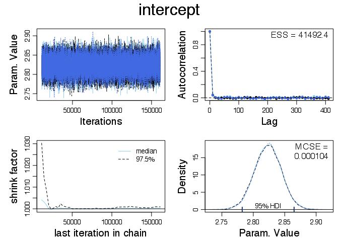
The top right ‘Param. Value’ plot shows, by inspection, that the three chains have all formed a stationary time series that overlap. This is an intuitive indication that they have converged, although it doesn’t guarantee it since all the chains could be in completely the wrong place. However this is unlikely and it is looking good that the samples are representative.
The auto correlation plot shows auto correlation at different lags for each chain. There is very little and this indicates that the Gibbs sampler has done a good job of exploring the possible parameters. This is another good indication of the samples being representative. Since there is no auto correlation the effective sample size is very close to the actual sample size. It is worth noting that there was a lot of auto correlation for the intercept when I ran the same model with 20,000 iterations and no thinning. In order to remove the autocorrelation thinning was added and the sampling became less efficient.
The shrink factor plot on the bottom left is probably the most involved so I will keep it brief. It compares the within chain and the between chain variance. See ?gelman.diag in R for more details! Apparently a good heuristic is that there is trouble if the value is greater than 1.1.
The final plot in the lower right hand corner shows density plots of each chain. They overlap which again indicates that the chains converged. The Monte Carlo standard error (MCSE) is the standard error of the mean of the parameter but with the effective sample size taken into account. We can see that the uncertainty for the intercept parameter is small and we can be happy that we understand the accuracy of the estimate.
Here is the home_adv diagnostic plot:
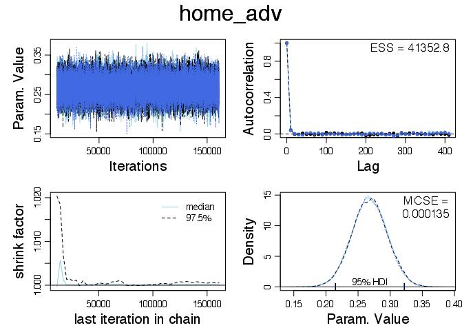
Again everything looks in order and we can see that we expect the mean value of home_adv to be around 0.268 with 0 well outside the HDI. Since we have
this means we also have
\begin{align} \theta^h_{ij} & = e^{intercept + home\_adv + att_i + def_j} \newline & = e^{intercept}e^{home\_adv}e^{att_i+def_j} \newline & = e^{home\_adv}(e^{intercept}e^{att_i+def_j}) \newline & = e^{home\_adv}\theta^a_{ji} \end{align}
Home advantage multiplies the teams scoring rate by a factor of \(e^{0.268} \simeq 1.307347\). So we expect that the home team will score roughly 31% more points on average then they would if the match was being played in the other teams ground. Exchanging home advantage can lead to a very different game!
The other 26 diagnostic plots look good, so I won’t include them here.
Comparing Teams
A nice plot that is generated in both the blog posts and article mentioned at the beginning is one of attacking parameters vs defensive parameters for each team. It required a good bit of wrangling to get a data.table in the correct shape.
# plot att def params against each other for each team with a label
# first get the means
x.1.summ <-cbind(summary(pro12.mcmc[[1]])$statistics, HPDinterval(pro12.mcmc[[1]], prob=0.95))
dt.param <- as.data.table(x.1.summ)
dt.param[,param:=rownames(x.1.summ)]

# It would be good to have all the parameters in att, def and misc. So search for the correct rows
# and then subset.
param.att <- dt.param[,grepl('att_',param)]
param.def <- dt.param[,grepl('def_',param)]
dt.param.att <- dt.param[param.att,]
dt.param.def <- dt.param[param.def,]
dt.param.nonteam <- dt.param[!(param.def | param.att),]
setkey(dt.param.nonteam,param)

# make the column names have att or def in them
setnames(dt.param.att,paste0('att.',tolower(sub('\\s+','.',names(dt.param.att)))))
setnames(dt.param.def,paste0('def.',tolower(sub('\\s+','.',names(dt.param.def)))))

# include team ids in param.att and param.def
dt.param.att[,team.id := as.integer(str_extract(att.param, '[0-9]+'))]
dt.param.def[,team.id := as.integer(str_extract(def.param, '[0-9]+'))]

# add the team names to the att dt
setkey(dt.param.att, team.id)
setkey(dt.param.def, team.id)
setkey(teams,team.id)
dt.param.att[,team := teams[J(team.id),team]]
# Nice to have the columns in an intuitive order
setcolorder(dt.param.att,
            colnames(dt.param.att)[c(ncol(dt.param.att),
                                     ncol(dt.param.att)-1,
                                     1:(ncol(dt.param.att)-2))])

# merge the dt on team.id
dt.param.team <- dt.param.att[dt.param.def,list(team,
                                             att.mean,
                                             att.lower,
                                             att.upper,
                                             def.mean,
                                             def.lower,
                                             def.upper )]
After all of that dt.param.team looks like this (pity about the wrapping)
print(dt.param.team)## team att.mean att.lower att.upper
## 1: Connacht Rugby 0.130112218 0.046021786 0.211093136
## 2: Edinburgh Rugby -0.094816733 -0.184117673 -0.004242146
## 3: Ulster Rugby 0.073636151 -0.013461072 0.155906406
## 4: Glasgow Warriors 0.216221366 0.135225674 0.295563996
## 5: Munster Rugby 0.034583893 -0.052002538 0.121044310
## 6: Cardiff Blues 0.205628477 0.126857231 0.288949864
## 7: Newport Gwent Dragons -0.201697228 -0.298713593 -0.105452369
## 8: Scarlets 0.080120748 -0.003831379 0.166508563
## 9: Benetton Treviso -0.271023734 -0.375352694 -0.174491361
## 10: Leinster Rugby 0.009037427 -0.076904997 0.096308457
## 11: Ospreys 0.105390522 0.021731201 0.192506379
## 12: Zebre Rugby -0.287193106 -0.390331354 -0.184395721
## def.mean def.lower def.upper
## 1: -0.05355414 -0.144713406 0.03775693
## 2: -0.17417483 -0.269849299 -0.07873939
## 3: -0.32667515 -0.432325480 -0.22262591
## 4: -0.10891475 -0.203904441 -0.01497540
## 5: -0.03574945 -0.128583933 0.05303158
## 6: 0.07764737 -0.009725686 0.16271203
## 7: 0.10492655 0.021809923 0.18776867
## 8: 0.05893814 -0.026165294 0.14845880
## 9: 0.31872284 0.243027427 0.39715170
## 10: -0.38796862 -0.490550693 -0.27820982
## 11: 0.05487715 -0.035363688 0.14120761
## 12: 0.47192489 0.401528623 0.54678271We can create the plot now!
# Plot the attack and defence parameters
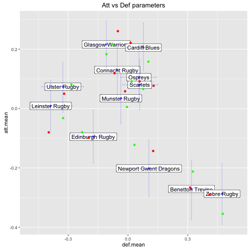
ggplot(dt.param.team,aes(x=def.mean, y=att.mean)) +
geom_label(aes(label=team, x=def.mean, y=att.mean),size=4) +
geom_point(color='blue', alpha=0.7) +
geom_errorbar(aes(x=def.mean, ymin=att.lower, ymax=att.upper), alpha=0.5, color='blue') +
geom_errorbarh(aes(y=att.mean, xmin=def.lower, xmax=def.upper), alpha=0.5, color='blue') +
ggtitle('Att vs Def parameters')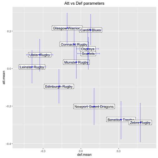
A notable observation is that this plot looks very similar to the plot of points for vs points against that we created at the beginning.

This is probably no surprise but what have we gained? Well a 95% HDI for both the attacking and defensive parameter of each team is also included. So now, in addition to the expected means, we also understand the uncertainty of the underlying attacking and defensive strengths of the teams.
Comparing the two plots is also valuable from a validation point of view - if they looked different it might indicate something had gone wrong!
Simulation
With an understanding of uncertainty we can perform simulations and figure out who is likely to win the Pro 12 Grand Final. Of course the only information the model has are the results in the league preceding the semi-finals and final. There are other factors that might be included in a more complex model e.g. injuries to key players.
When using the outputs of MCMC to simulate it is important to understand that each of the parameter values in each sample of a chain are only valid when considered together. For instance here are two different samples from the first chain overlayed on the plot above - one as red dots and the other as green.
Obviously it is not always clear which dots belongs to each team, but the point is to observe how the shape of the overall landscape can change. The parameters from each sample are bound together, so when we sample from the distributions we must respect this. Never mix values from different samples of the chain.
My code for simulating the playoffs is below. A couple of things to note are:
-
if there was a draw I just let the teams play again since the model has no concept of extra time etc.
-
The Grand Final is at a neutral venue which the model also doesn’t understand. So I played the game twice with each team playing at home once. I then took the aggregate score. I thought about setting the
home_advparameter to zero but I’d worry this would upset the balance of the model.
SimOneGame <- function(mcmc.obj, home.id, away.id, neutral=FALSE, s=NULL) {
  # First choose sample
  if (is.null(s)) {
    s <- sample(nrow(mcmc.obj[[1]]),1)
  }

  # get the attack and defence parameters
  home.att.col <- which(colnames(mcmc.obj[[1]]) == paste0('att_centered[',home.id,']'))
  away.att.col <- which(colnames(mcmc.obj[[1]]) == paste0('att_centered[',away.id,']'))
  home.def.col <- which(colnames(mcmc.obj[[1]]) == paste0('def_centered[',home.id,']'))
  away.def.col <- which(colnames(mcmc.obj[[1]]) == paste0('def_centered[',away.id,']'))

  this.game.params <- mcmc.obj[[1]][s,]

  home.att <- this.game.params[home.att.col]
  away.att <- this.game.params[away.att.col]
  home.def <- this.game.params[home.def.col]
  away.def <- this.game.params[away.def.col]

  # Also need intercept and home_adv
  home.adv.col <- which(colnames(mcmc.obj[[1]]) == 'home_adv')
  intercept.col <- which(colnames(mcmc.obj[[1]]) == 'intercept')

  home.adv <- this.game.params[home.adv.col]
  intercept <- this.game.params[intercept.col]

  # Now calc the thetas
  if(!neutral) {
    home.theta <- exp(intercept + home.adv + home.att + away.def)
  } else {
    home.theta <- exp(intercept + home.att + away.def)
  }

  away.theta <- exp(intercept + away.att + home.def)

  score <- rpois(1,home.theta)
  score[2] <- rpois(1,away.theta)

  if (score[1] > score[2])
    return(list(winner.id=home.id, score=score))

  if (score[1] == score[2])
    return(list(winner.id=0, score=score))

  if (score[1] < score[2])
    return(list(winner.id=away.id, score=score))
}

SimOnePlayOff <- function(mcmc.obj, top.four) {
  s <- sample(nrow(mcmc.obj[[1]]),1)

  # play games until there is no draw, in lieu of extra time etc.
  repeat {
    semi.final.one <- SimOneGame(mcmc.obj, home.id=top.four[1], away.id=top.four[4], s=s)
    if (semi.final.one$winner.id != 0)
      break
  }

  repeat {
    semi.final.two <- SimOneGame(mcmc.obj, home.id=top.four[2], away.id=top.four[3], s=s)
    if (semi.final.two$winner.id != 0)
      break
  }

  # the final is now played in a neutral location, which is annoying
  # as there is no concept of neutral location in the model.
  # So play the game twice, switching the home and away teams,
  # and decide result on aggregate.
  repeat {
    final1 <- SimOneGame(mcmc.obj, home.id=semi.final.one$winner.id, away.id=semi.final.two$winner.id, s=s)
    final2 <- SimOneGame(mcmc.obj, home.id=semi.final.two$winner.id, away.id=semi.final.one$winner.id, s=s)
    # score[1] here will be semi.final.one
    score <- final1$score  + rev(final2$score)

    if (score[1] != score[2])
      break
  }

  # We can't have draws here
  if (score[1] > score[2])
    return(list(winner=semi.final.one$winner.id, path=paste(semi.final.one$winner.id,
                                                             semi.final.two$winner.id,
                                                             semi.final.one$winner.id,
                                                             sep='-')))

  if (score[1] < score[2])
    return(list(winner=semi.final.two$winner.id, path=paste(semi.final.one$winner.id,
                                                            semi.final.two$winner.id,
                                                            semi.final.two$winner.id,
                                                            sep='-')))

}
The OnePlayoff function plays one iteration of the semi-finals and the finals. Its top.four argument specifies the team.id of the teams that finished in the top four and in what order. Note that the sample s is set at the start of this function and passed to the SimOneGame function when required.
Now to run some simulations based on the top four of the league:
- Leinster Rugby
- Connacht Rugby
- Glasgow Warriors
- Ulster Rugby
Note that the competition rules say that the top 2 get home advantage. This means that the semi-finals are
- Leinster Rugby vs Ulster Rugby (i.e. 1 vs 4)
- Connacht Rugby vs Glasgow Warriors (i.e. 2 vs 3)
 Pro12Simulations <- function(teams, mcmc.obj, top.four.names, n=5000) {
  setkey(teams, team)
  # Top four teams in order
  top.four <- data.table(team=top.four.names
                         ,table.position=1:4)
  dt.top.four <- teams[top.four, ]
  top.four.ids <- dt.top.four[order(table.position),team.id]
  # 5000 simulations of playoffs and use put it in a data.table
  res <- lapply(1:n, function(z) SimOnePlayOff(mcmc.obj, top.four.ids))
  dt.winner <- data.table(team.id=sapply(res, function(x) x$winner))
  dt.path <- data.table(path=sapply(res, function(x) x$path))
  # Get the proportion of simulations that each team won the Grand Final.
  dt.winner <- dt.winner[,list(proportion.winner=.N/nrow(dt.winner)), by=team.id]
  dt.path <- dt.path[,list(proportion.path=.N/nrow(dt.path)), by=path]
  setkey(dt.winner, team.id)
  setkey(dt.top.four, team.id)
  # Return a data table of
  list(dt.winner.proportion=dt.top.four[dt.winner,], dt.path.proportion=dt.path)
 }

top.four.names <- c('Leinster Rugby', 'Connacht Rugby', 'Glasgow Warriors', 'Ulster Rugby')
playoff.sim.results <- Pro12Simulations(teams, pro12.mcmc, top.four.names)

ggplot(playoff.sim.results$dt.winner.proportion) +
  geom_bar(aes(team, proportion.winner), stat="identity") +
   geom_text(aes(x=team, y= proportion.winner, label=proportion.winner), vjust=-0.5) +
  ylim(c(0,1)) +
  ggtitle('Simulation Results')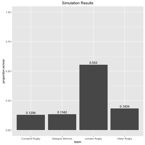
So given just the results from the league and the final configuration of the top four the model says there is a 55% chance that Leinster will win the Pro 12. We talked about home advantage being very important above, and given that the top two teams in the league get home semi-finals it might be interesting to see how things would change if the top four configuration were different. For instance what if Connacht and Glasgow swapped positions i.e.
- Leinster Rugby
- Glasgow Warriors
- Connacht Rugby
- Ulster Rugby
Then we get the following
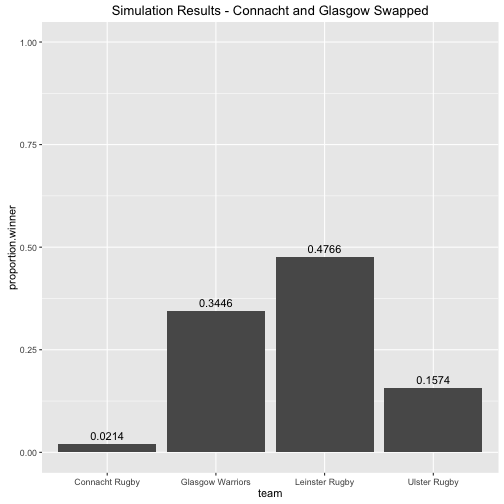
Things change quite dramatically! Home advantage is crucial.
The final
In the intro I mentioned that I didn’t get this post online before the semi-finals. One benefit of this is that we know that Leinster beat Ulster and Connacht beat Glasgow. The SimOnePlayoff function above returns the path of the final result. So for example 10-1-1 indicates team.id 10 won the first semi-final, team.id 1 won the second, and then team.id 1 ultimately won the Grand Final against team.id 10. Leinster have team.id 10 and Connacht have team.id 1, so let’s look at the distribution of the paths.
playoff.sim.results$dt.path.proportion## path proportion.path
## 1: 10-1-10 0.3912
## 2: 3-1-1 0.0322
## 3: 10-1-1 0.0972
## 4: 3-1-3 0.1302
## 5: 10-4-4 0.1026
## 6: 10-4-10 0.1618
## 7: 3-4-4 0.0316
## 8: 3-4-3 0.0532We can see that a Leinster Connacht Grand Final was always the most likely outcome accounting for around 50% of the finals in the 5,000 simulations. Of these finals, Leinster won roughly 4 of every 5.
Personally, I think the final will be much closer than this analysis suggests. It is important to note that the model doesn’t have any concept of time. Results at the start of the season are given the same importance as results at the end. Therefore the parameters being estimated are an average from across the season. Given the volatile nature of sport (injuries etc.) this is not the most prudent approach when understanding the uncertainty in match results. However it is a fun exercise none the less!